Working with Zonation projects

1. Zonation projects and zonator classes

The following examples will use the basic Zonation tutorial data as shipped with the zdat package. The input and output files in the tutorial package are arranged in a layout that has a specific logic behind it. In Zonation jargon, everything within the root folder basic is consider to belong to the same project (see figure below). A project constitutes of one or several variants. Each variant is an individual Zonation run with specific input biodidiversity features (defined in 01.spp) and input parameters (defined in 01.dat). All the configuration files needed for a run are specified in a Windows batch file (01_core_area_zonation.bat). For convience and clarity, input files required are placed in a subfolder named after the variant. After the variant is run (in Zonation), the outputs of the variant are placed in another subfolder (e.g. 01/01_out/).

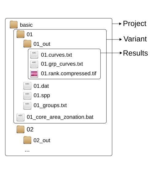
Folder structure

All in all, the tutorial data has one project which has five variants (not all are shown in the figure above for brevity). Note that these specification are just a useful convention and are not at all required by Zonation (or zonator)! Note also that these specification are related to Zonation itself. Conceptually, zonator uses the same terminology and the S4 classes in zonator follow the same logic. zonator provides a two functions create_zproject() and load_zproject() that can be used to:

Create a new Zonation project on the file system (create_zproject())
Create zonator project based on existing Zonation project (load_zproject())

load_zproject() works by parsing real input files on your file system (needed by Zonation) into R data structures. Formally, load_zproject() creates a new instance (object) of class Zproject with has specific attributes representing the Zonation project on the file system. Each variant (see above) is parsed into an instance of class Zvariant. If a variant already has results produced by Zonation, then these are parsed and mapped into an instance of class Zresults.

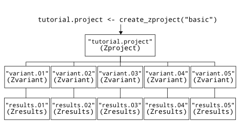
Class structure

Each class has specific methods that can be used to get and set attributes, see documentation and the packages vignettes for more detailed description.

2. Create a new Zonation project

As mentioned above, zonator packages provides function create_zproject() that can be used to create all the necessary files and folders for a new Zonation project. Let’s take a closer look:

library(zonator)

# Create a (temporary) path to a new project. Basename component of this path
# will also be the name of the project.
project_path <- file.path(tempdir())

# Define the names of the variants within the project
variant_names <- c("01_variant", "02_variant", "03_variant")

# Create a new project from scratch. Note that since we do not provide any 
# template file paths (for the .spp and .dat files), the templates shipped
# with the tutorial data will be used.
create_zproject(name = "test_project", dir = project_path,
                variants = variant_names)

If you ran these examples on your own computer, you can now open path defined in project_path in your file browser to see what was created. Another useful option for create_zproject() is that it can scan the content of a given directory for raster (input biodiversity feature) files and construct a spp-file based on the file listing. Let’s create a new project from scratch using input raster files shipped with the Zonation tutorial as a basis for the spp file. Since the input folder contains more rasters than just biodiversity files, we’ll be using a file name filter. Note that we are still usingthe template .dat-file.

# Directory containing the input raster files
input_raster_dir <- system.file("extdata/test_project/data", package="zonator")
new_project <- create_zproject(name = "test_project", dir = project_path,
                               variants = variant_names,
                               spp_template_dir = input_raster_dir,
                               spp_file_pattern = "^species[0-9].tif$")

You can give extra arguments to create_zproject() that will be passed on to creating the spp file. E.g. if you would want the set different weights to your biodiversity features, you could do the following:

new_project <- create_zproject(name = "test_project", dir = project_path, 
                               variants = variant_names,
                               spp_template_dir = input_raster_dir,
                               spp_file_pattern = "^species[0-9].tif$",
                               weight = c(1, 1, 1, 2, 3, 2, 1)

Be careful with setting the weights (or other spp-file parameters such as the alpha value), because no checking is being done!

3. Create zonator project based on existing data

Alternatively, all the information contained within an existing Zonation project can be parsed into R data structures. The tutorial data is not distributed with zonator, but in a separate package zdat. You can - and must if you want to run the examples below - install the package by:

library(devtools)
devtools::install_github("cbig/zdat")

The tutorial data include results of the tutorial runs so there is no need to run the variants in order to inspect the results. In case you do want to rerun the variants and you have Zonation installed in your system do so by running the following code. Otherwise just skip this code section.

library(zonator)

setup.dir <- system.file("extdata/basic", package = "zdat")

# Get all the bat-files
bat.files <- list.files(setup.dir, "\\.bat$", full.names = TRUE)
## 
## # Run all the runs
## #for (bat.file in bat.files) {
## #  run_bat(bat.file)
## #}
##

You can create a new zonator project based on existing data by using load_zproject():

tutorial.project <- load_zproject(setup.dir)

Pro tip! In case you have a complex Zonation project and want to keep track which files are being read in while creating zproject, you can do load_zproject(setup.dir, debug=TRUE) in order to enable logging of file reading sequence.

zonator also includes a utility function opendir() which takes a zproject object as an argument and opens the file system folder containing the setup files:

opendir(tutorial.project)

2. Working with variants

Individual variants (i.e. runs) can be extracted form the project using an index number. nvariants() will tell how many variants are included in the project.

nvariants(tutorial.project)

## [1] 6

variant.1 <- get_variant(tutorial.project, 1)

Using an index number such as 1 is one option, but you can also use the name of the variant. By default, zonator will assign the name of bat-file used to run the run as a name, without the “.bat” extensions of course. names() will print the names of all the variants. Name can also be used to extract a variant.

names(tutorial.project)

## [1] "01" "02" "03" "04" "05" "07"

# Get first variant, 01_core_area_zonation
variant.caz <- get_variant(tutorial.project, "01")

Each variant object is an instance of class Zvariant and have a suite of useful methods for dealing with data parsed from various Zonation input files.

2.1 spp data

Zonation spp-file is one of the mandatory input files that always needs to be in place and thus all variants have one. When a new Zvariant instance is created the associated spp file is automatically parsed into it. All the spp data (with group code column if available) can be retrieved using sppdata():

sppdata(variant.caz)

##   weight alpha bqp bqp_p cellrem             filepath     name group
## 1      1  1.00   1     1       1 ../data/species1.tif species1     1
## 2      1  0.50   1     1       1 ../data/species2.tif species2     2
## 3      1  0.25   1     1       1 ../data/species3.tif species3     2
## 4      1  0.75   1     1       1 ../data/species4.tif species4     1
## 5      1  0.50   1     1       1 ../data/species5.tif species5     2
## 6      1  1.50   1     1       1 ../data/species6.tif species6     1
## 7      1  1.00   1     1       1 ../data/species7.tif species7     1

You can check the number of features in spp file by using method nfeatures():

nfeatures(variant.caz)

## [1] 7

Zvariant objects have a couple of other convenience functions for quickly accessing columns in the spp file. For example, sppweights() can be used to extract the weight column in spp file:

# Note that all biodiversity features (species) have an equal weight of 1
sppweights(variant.caz)

## [1] 1 1 1 1 1 1 1

Feature names from the spp file/data can be accessed directly by using method featurenames().

featurenames(variant.caz)

## [1] "species1" "species2" "species3" "species4" "species5" "species6" "species7"

The generated names are not necessarily very informative and can be changed to new values. Remember that the names need to be valid data frame column names (zontor will try to fix these even if you don’t).

featurenames(variant.caz) <- c("Koala", "Masked.owl", "Powerful.owl",
                             "Tiger.quoll", "Sooty.owl", "Squirrel.glider",
                             "Yellow-bellied.glider")
featurenames(variant.caz)

## [1] "Koala"                 "Masked.owl"            "Powerful.owl"          "Tiger.quoll"          
## [5] "Sooty.owl"             "Squirrel.glider"       "Yellow-bellied.glider"

# Or all the spp data
sppdata(variant.caz)

##   weight alpha bqp bqp_p cellrem             filepath                  name group
## 1      1  1.00   1     1       1 ../data/species1.tif                 Koala     1
## 2      1  0.50   1     1       1 ../data/species2.tif            Masked.owl     2
## 3      1  0.25   1     1       1 ../data/species3.tif          Powerful.owl     2
## 4      1  0.75   1     1       1 ../data/species4.tif           Tiger.quoll     1
## 5      1  0.50   1     1       1 ../data/species5.tif             Sooty.owl     2
## 6      1  1.50   1     1       1 ../data/species6.tif       Squirrel.glider     1
## 7      1  1.00   1     1       1 ../data/species7.tif Yellow-bellied.glider     1

2.2 Groups

Notice that data frames returned by sppdata() in previous examples already had a column called “group”. This is because all tutorial variants have groups enabled by default. If a variant doesn’t use groups, then this column will be missing.

Group identities in Zonation input file are coded with integer values. Method groups() will return just this integer vector:

groups(variant.caz)

## [1] 1 2 2 1 2 1 1

Groups can also have more informative names attached to them by using method groupnames(). Even if you haven’t names the groups used (Zonation does not have a concept of named groups), generic group names “group1”, “group2” etc. will automatically be created for Zvariant objects with groups enabled.

# By default, generic group names are used
groupnames(variant.caz)

## [1] "group1" "group2"

The format for setting (mapping) group names is strict and involves a named character vector in which (column) names correspond to integer group codes and character elements the group names to be assigned:

# Construct a group name mapping using a named character vector
groupnames(variant.caz) <- c("1" = "mammals", "2" = "owls")
groupnames(variant.caz)

## [1] "mammals" "owls"

Now group 1 is labeled “mammals” and group 2 is labeled “owls”. Note that sppdata() has an optional argument group.names that can be set to TRUE if group names are preferable to group codes.

sppdata(variant.caz, group.names = TRUE)

##   weight alpha bqp bqp_p cellrem             filepath                  name group.name
## 1      1  1.00   1     1       1 ../data/species1.tif                 Koala    mammals
## 2      1  0.50   1     1       1 ../data/species2.tif            Masked.owl       owls
## 3      1  0.25   1     1       1 ../data/species3.tif          Powerful.owl       owls
## 4      1  0.75   1     1       1 ../data/species4.tif           Tiger.quoll    mammals
## 5      1  0.50   1     1       1 ../data/species5.tif             Sooty.owl       owls
## 6      1  1.50   1     1       1 ../data/species6.tif       Squirrel.glider    mammals
## 7      1  1.00   1     1       1 ../data/species7.tif Yellow-bellied.glider    mammals

In addition to changing the group names, you can change the groups themselves as well. In the previous examples we had two groups named “mammals” (group code = 1) and “owls” (group code = 2). Belonging to either one of these groups is controlled by the group ID code (an integer number) that can be accessed by groups():

groups(variant.caz)

## [1] 1 2 2 1 2 1 1

Method groups() can be used to set the group ID codes and thus the grouping. Let’s say you want to split owls into two sub-groups called “big.owls” (group code = 2) containing the Sooty owl and the Masked Owl and “small.owls” (group code = 3) containing the Powerful owl. Take again a look at the spp data:

sppdata(variant.caz)

##   weight alpha bqp bqp_p cellrem             filepath                  name group
## 1      1  1.00   1     1       1 ../data/species1.tif                 Koala     1
## 2      1  0.50   1     1       1 ../data/species2.tif            Masked.owl     2
## 3      1  0.25   1     1       1 ../data/species3.tif          Powerful.owl     2
## 4      1  0.75   1     1       1 ../data/species4.tif           Tiger.quoll     1
## 5      1  0.50   1     1       1 ../data/species5.tif             Sooty.owl     2
## 6      1  1.50   1     1       1 ../data/species6.tif       Squirrel.glider     1
## 7      1  1.00   1     1       1 ../data/species7.tif Yellow-bellied.glider     1

What needs to be done is to change the group ID for the Powerful owl so that the group ID vector is changed into 1, 2, 3, 1, 2, 1, 1. So do the following:

groups(variant.caz) <- c(1, 2, 3, 1, 2, 1, 1)
# Check the group ID codes
groups(variant.caz)

## [1] 1 2 3 1 2 1 1

Note that after you change the group ID codes all the group names you may have assigned get lost and are again replaced by generic “group1”, “group2” etc. You will have to manually set the group names again:

# Using generic group names after the group IDs have been changed
groupnames(variant.caz)

## [1] "group1" "group2" "group3"

# Construct a new group names mapping
groupnames(variant.caz) <- c("1" = "mammals", "2" = "big.owls",
                             "3" = "small.owls")
groupnames(variant.caz)

## [1] "mammals"    "big.owls"   "small.owls"

or check the whole spp data with group names:

sppdata(variant.caz, group.names = TRUE)

##   weight alpha bqp bqp_p cellrem             filepath                  name group.name
## 1      1  1.00   1     1       1 ../data/species1.tif                 Koala    mammals
## 2      1  0.50   1     1       1 ../data/species2.tif            Masked.owl   big.owls
## 3      1  0.25   1     1       1 ../data/species3.tif          Powerful.owl small.owls
## 4      1  0.75   1     1       1 ../data/species4.tif           Tiger.quoll    mammals
## 5      1  0.50   1     1       1 ../data/species5.tif             Sooty.owl   big.owls
## 6      1  1.50   1     1       1 ../data/species6.tif       Squirrel.glider    mammals
## 7      1  1.00   1     1       1 ../data/species7.tif Yellow-bellied.glider    mammals